Examples
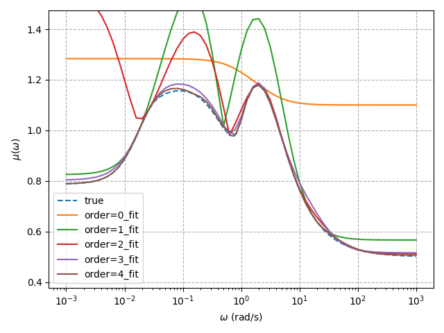
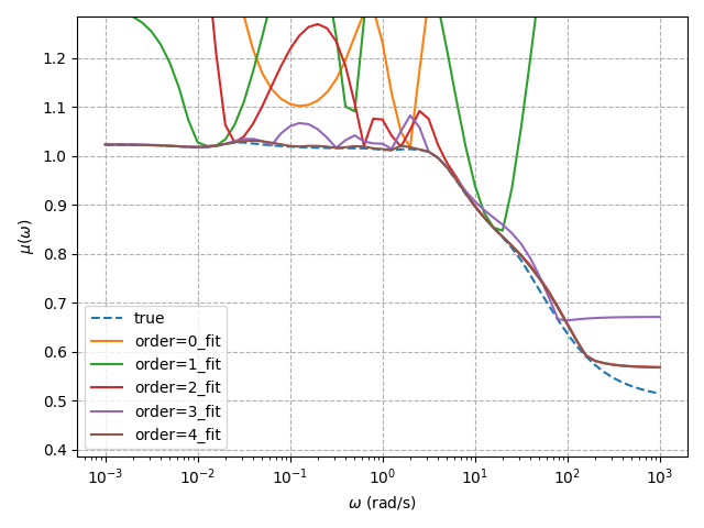
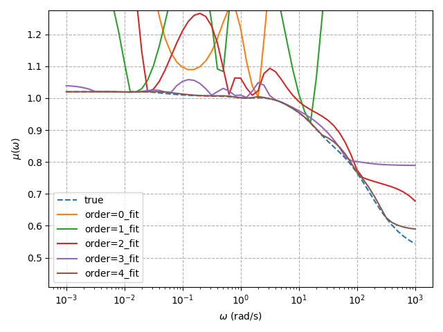
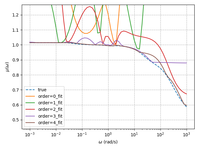
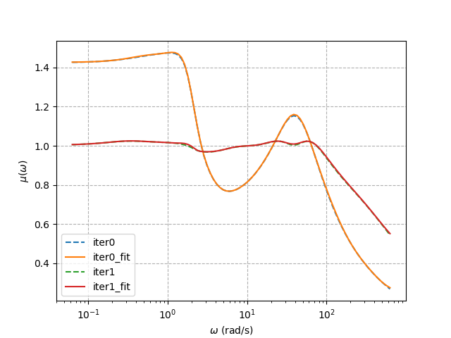
In all the examples on this page, three iterations with 4th order D-scale fits are used to reproduce the example from [SP06], Table 8.2 (p. 325). Each example recovers the same result, but with a different way to specify the D-scale fit orders.
This example is quite numerically challenging, so if you encounter a solver error, you may need to experiment with solver tolerances.
D-K iteration with fixed fit order
In this example, the number of iterations is fixed to 3 and the order is fixed to 4.
"""D-K iteration with fixed number of iterations and fit order."""
import numpy as np
from matplotlib import pyplot as plt
import dkpy
def example_dk_iter_fixed_order():
"""D-K iteration with fixed number of iterations and fit order."""
eg = dkpy.example_skogestad2006_p325()
dk_iter = dkpy.DkIterFixedOrder(
controller_synthesis=dkpy.HinfSynSlicot(),
structured_singular_value=dkpy.SsvLmiBisection(n_jobs=1),
d_scale_fit=dkpy.DScaleFitSlicot(),
n_iterations=3,
fit_order=4,
)
omega = np.logspace(-3, 3, 61)
# Alternative MATLAB block structure description
# uncertainty_structure = dkpy.UncertaintyBlockStructure(
# [[1, 1], [1, 1], [2, 2]]
# )
uncertainty_structure = [
dkpy.ComplexFullBlock(1, 1),
dkpy.ComplexFullBlock(1, 1),
dkpy.ComplexFullBlock(2, 2),
]
K, N, mu, iter_results, info = dk_iter.synthesize(
eg["P"],
eg["n_y"],
eg["n_u"],
omega,
uncertainty_structure,
)
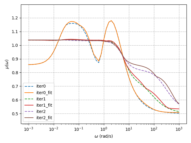
print(f"mu={mu}")
fig, ax = plt.subplots()
for i, ds in enumerate(iter_results):
dkpy.plot_mu(ds, ax=ax, plot_kw=dict(label=f"iter{i}"))
ax = None
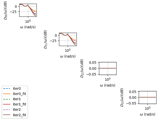
for i, ds in enumerate(iter_results):
fig, ax = dkpy.plot_D(ds, ax=ax, plot_kw=dict(label=f"iter{i}"))
plt.show()
if __name__ == "__main__":
example_dk_iter_fixed_order()
Output:
mu=1.0368156433105469
D-K iteration with list of fit orders
In this example, the orders are specified in a list. They can be specified manually for each entry of the D matrix, or they can all be set to the same integer.
"""D-K iteration with fixed number of iterations and fit order."""

import numpy as np
from matplotlib import pyplot as plt

import dkpy


def example_dk_iter_list_order():
    """D-K iteration with a list of fit orders."""
    eg = dkpy.example_skogestad2006_p325()

    dk_iter = dkpy.DkIterListOrder(
        controller_synthesis=dkpy.HinfSynSlicot(),
        structured_singular_value=dkpy.SsvLmiBisection(),
        d_scale_fit=dkpy.DScaleFitSlicot(),
        # fit_orders=[4, 4, 4],  # <- an alternative
        fit_orders=[
            [4, 4, 0],
            [4, 4, 0],
            [4, 4, 0],
        ],
    )

    omega = np.logspace(-3, 3, 61)
    # Alternative MATLAB block structure description
    # uncertainty_structure = dkpy.UncertaintyBlockStructure(
    #     [[1, 1], [1, 1], [2, 2]]
    # )
    uncertainty_structure = [
        dkpy.ComplexFullBlock(1, 1),
        dkpy.ComplexFullBlock(1, 1),
        dkpy.ComplexFullBlock(2, 2),
    ]
    K, N, mu, iter_results, info = dk_iter.synthesize(
        eg["P"],
        eg["n_y"],
        eg["n_u"],
        omega,
        uncertainty_structure,
    )

    print(f"mu={mu}")

    fig, ax = plt.subplots()
    for i, ds in enumerate(iter_results):
        dkpy.plot_mu(ds, ax=ax, plot_kw=dict(label=f"iter{i}"))

    ax = None
    for i, ds in enumerate(iter_results):
        fig, ax = dkpy.plot_D(ds, ax=ax, plot_kw=dict(label=f"iter{i}"))

    plt.show()


if __name__ == "__main__":
    example_dk_iter_list_order()
Output:
mu=1.0368156433105469


D-K iteration with automatically selected fit orders
In this example, multiple fit orders are attempted up to a maximum, and the one with the lowest relative error is selected.
"""D-K iteration with fixed number of iterations and fit order.
If you don't have access to MOSEK, see the ``DkIteration`` object settings from
the first two examples.
"""
import logging
import numpy as np
from matplotlib import pyplot as plt
import dkpy
logging.basicConfig(level=logging.INFO)
def example_dk_iter_auto_order():
"""D-K iteration automatically selected fit orders."""
eg = dkpy.example_skogestad2006_p325()
dk_iter = dkpy.DkIterAutoOrder(
controller_synthesis=dkpy.HinfSynLmi(
lmi_strictness=1e-7,
solver_params=dict(
solver="MOSEK",
eps=1e-8,
),
),
structured_singular_value=dkpy.SsvLmiBisection(
bisection_atol=1e-5,
bisection_rtol=1e-5,
max_iterations=1000,
lmi_strictness=1e-7,
solver_params=dict(
solver="MOSEK",
eps=1e-9,
),
n_jobs=1,
),
d_scale_fit=dkpy.DScaleFitSlicot(),
max_mu=1,
max_mu_fit_error=1e-2,
max_iterations=3,
max_fit_order=4,
)
omega = np.logspace(-3, 3, 61)
# Alternative MATLAB block structure description
# uncertainty_structure = dkpy.UncertaintyBlockStructure(
# [[1, 1], [1, 1], [2, 2]]
# )
uncertainty_structure = [
dkpy.ComplexFullBlock(1, 1),
dkpy.ComplexFullBlock(1, 1),
dkpy.ComplexFullBlock(2, 2),
]
K, N, mu, iter_results, info = dk_iter.synthesize(
eg["P"],
eg["n_y"],
eg["n_u"],
omega,
uncertainty_structure,
)
print(f"mu={mu}")
fig, ax = plt.subplots()
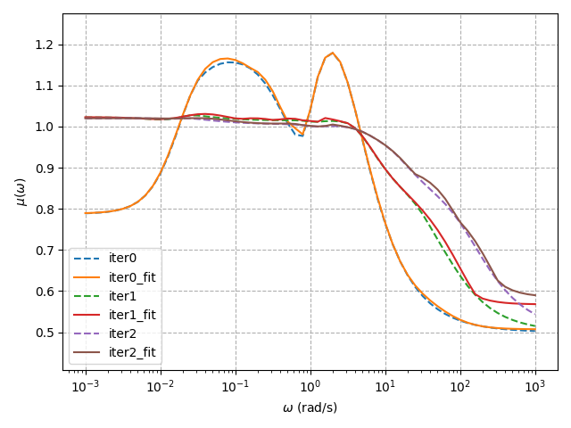
for i, ds in enumerate(iter_results):
dkpy.plot_mu(ds, ax=ax, plot_kw=dict(label=f"iter{i}"))
ax = None
for i, ds in enumerate(iter_results):
fig, ax = dkpy.plot_D(ds, ax=ax, plot_kw=dict(label=f"iter{i}"))
plt.show()
if __name__ == "__main__":
example_dk_iter_auto_order()
Output:
INFO:DkIterAutoOrder:Iteration: 0, mu: 1.1792182922363281
INFO:DkIterAutoOrder:Order 0 relative error: 0.5066119732511977
INFO:DkIterAutoOrder:Order 1 relative error: 0.3356881131800033
INFO:DkIterAutoOrder:Order 2 relative error: 0.643462672042705
INFO:DkIterAutoOrder:Order 3 relative error: 0.031649076289004166
INFO:DkIterAutoOrder:Order 4 relative error: 0.012866875729555234
INFO:DkIterAutoOrder:Reached max fit order, selecting order 4
INFO:DkIterAutoOrder:Iteration: 1, mu: 1.0274028778076172
INFO:DkIterAutoOrder:Order 0 relative error: 9.780743577129419
INFO:DkIterAutoOrder:Order 1 relative error: 1.4151255816143613
INFO:DkIterAutoOrder:Order 2 relative error: 8.507402105789147
INFO:DkIterAutoOrder:Order 3 relative error: 0.15216618301078452
INFO:DkIterAutoOrder:Order 4 relative error: 0.05185270360448734
INFO:DkIterAutoOrder:Reached max fit order, selecting order 4
INFO:DkIterAutoOrder:Iteration: 2, mu: 1.0203123092651367
INFO:DkIterAutoOrder:Order 0 relative error: 30.002715934629506
INFO:DkIterAutoOrder:Order 1 relative error: 4.172954343879354
INFO:DkIterAutoOrder:Order 2 relative error: 9.026259323212026
INFO:DkIterAutoOrder:Order 3 relative error: 0.24098884948353583
INFO:DkIterAutoOrder:Order 4 relative error: 0.04541136749668787
INFO:DkIterAutoOrder:Reached max fit order, selecting order 4
INFO:DkIterAutoOrder:Iteration: 3, mu: 1.0144329071044922
INFO:DkIterAutoOrder:Iteration terminated: reached maximum number of iterations
INFO:DkIterAutoOrder:Iteration complete
mu=1.0144329071044922

D-K iteration with interactively selected fit orders
In this example, the user is prompted to select a D-scale fit order at each iteration. The user is shown the frequency-by-frequency and fit structured singular value plots at each iteration.
"""D-K iteration with fixed number of iterations and fit order.

If you don't have access to MOSEK, see the ``DkIteration`` object settings from
the first two examples.
"""

import numpy as np
from matplotlib import pyplot as plt

import dkpy


def example_dk_iter_interactive():
    """D-K iteration with interactively selected fit orders."""
    eg = dkpy.example_skogestad2006_p325()

    dk_iter = dkpy.DkIterInteractiveOrder(
        controller_synthesis=dkpy.HinfSynLmi(
            lmi_strictness=1e-7,
            solver_params=dict(
                solver="MOSEK",
                eps=1e-8,
            ),
        ),
        structured_singular_value=dkpy.SsvLmiBisection(
            bisection_atol=1e-5,
            bisection_rtol=1e-5,
            max_iterations=1000,
            lmi_strictness=1e-7,
            solver_params=dict(
                solver="MOSEK",
                eps=1e-9,
            ),
        ),
        d_scale_fit=dkpy.DScaleFitSlicot(),
        max_fit_order=4,
    )

    omega = np.logspace(-3, 3, 61)
    # Alternative MATLAB block structure description
    # uncertainty_structure = dkpy.UncertaintyBlockStructure(
    #     [[1, 1], [1, 1], [2, 2]]
    # )
    uncertainty_structure = [
        dkpy.ComplexFullBlock(1, 1),
        dkpy.ComplexFullBlock(1, 1),
        dkpy.ComplexFullBlock(2, 2),
    ]
    K, N, mu, iter_results, info = dk_iter.synthesize(
        eg["P"],
        eg["n_y"],
        eg["n_u"],
        omega,
        uncertainty_structure,
    )

    print(f"mu={mu}")

    fig, ax = plt.subplots()
    for i, ds in enumerate(iter_results):
        dkpy.plot_mu(ds, ax=ax, plot_kw=dict(label=f"iter{i}"))

    ax = None
    for i, ds in enumerate(iter_results):
        fig, ax = dkpy.plot_D(ds, ax=ax, plot_kw=dict(label=f"iter{i}"))

    plt.show()


if __name__ == "__main__":
    example_dk_iter_interactive()
Prompt:
Close plot to continue...
Select order (<Enter> to end iteration): 4
Prompt:
Close plot to continue...
Select order (<Enter> to end iteration): 4
Prompt:
Close plot to continue...
Select order (<Enter> to end iteration): 4
Output:
Close plot to continue...
Select order (<Enter> to end iteration):
Iteration ended.
mu=1.0144329071044922


D-K iteration with a custom fit order selection method
In this example, a custom D-K iteration class is used to stop the iteration after 3 iterations of 4th order fits.
"""D-K iteration with fixed number of iterations and fit order.

If you don't have access to MOSEK, see the ``DkIteration`` object settings from
the first two examples.
"""

import numpy as np
from matplotlib import pyplot as plt

import dkpy


class MyDkIter(dkpy.DkIteration):
    """Custom D-K iteration class with interactive order selection."""

    def __init__(
        self,
        controller_synthesis,
        structured_singular_value,
        d_scale_fit,
    ):
        super().__init__(
            controller_synthesis,
            structured_singular_value,
            d_scale_fit,
        )
        self.my_iter_count = 0

    def _get_fit_order(
        self,
        iteration,
        omega,
        mu_omega,
        D_l_omega,
        D_r_omega,
        P,
        K,
        block_structure,
    ):
        print(f"Iteration {self.my_iter_count} with mu of {np.max(mu_omega)}")
        if self.my_iter_count < 3:
            self.my_iter_count += 1
            return 4
        else:
            return None


def example_dk_iter_custom():
    """D-K iteration with fixed number of iterations and fit order."""
    eg = dkpy.example_skogestad2006_p325()

    dk_iter = MyDkIter(
        controller_synthesis=dkpy.HinfSynLmi(
            lmi_strictness=1e-7,
            solver_params=dict(
                solver="MOSEK",
                eps=1e-8,
            ),
        ),
        structured_singular_value=dkpy.SsvLmiBisection(
            bisection_atol=1e-5,
            bisection_rtol=1e-5,
            max_iterations=1000,
            lmi_strictness=1e-7,
            solver_params=dict(
                solver="MOSEK",
                eps=1e-9,
            ),
            n_jobs=1,
        ),
        d_scale_fit=dkpy.DScaleFitSlicot(),
    )

    omega = np.logspace(-3, 3, 61)
    # Alternative MATLAB block structure description
    # uncertainty_structure = dkpy.UncertaintyBlockStructure(
    #     [[1, 1], [1, 1], [2, 2]]
    # )
    uncertainty_structure = [
        dkpy.ComplexFullBlock(1, 1),
        dkpy.ComplexFullBlock(1, 1),
        dkpy.ComplexFullBlock(2, 2),
    ]
    K, N, mu, iter_results, info = dk_iter.synthesize(
        eg["P"],
        eg["n_y"],
        eg["n_u"],
        omega,
        uncertainty_structure,
    )

    print(f"mu={mu}")

    fig, ax = plt.subplots()
    for i, ds in enumerate(iter_results):
        dkpy.plot_mu(ds, ax=ax, plot_kw=dict(label=f"iter{i}"))

    ax = None
    for i, ds in enumerate(iter_results):
        fig, ax = dkpy.plot_D(ds, ax=ax, plot_kw=dict(label=f"iter{i}"))

    plt.show()


if __name__ == "__main__":
    example_dk_iter_custom()
Output:
Iteration 0 with mu of 1.1792182922363281
Iteration 1 with mu of 1.0274028778076172
Iteration 2 with mu of 1.0203123092651367
Iteration 3 with mu of 1.0144329071044922
mu=1.0144329071044922


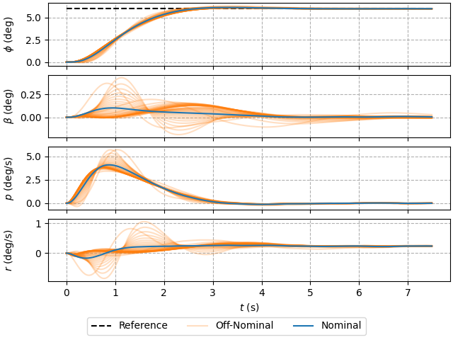
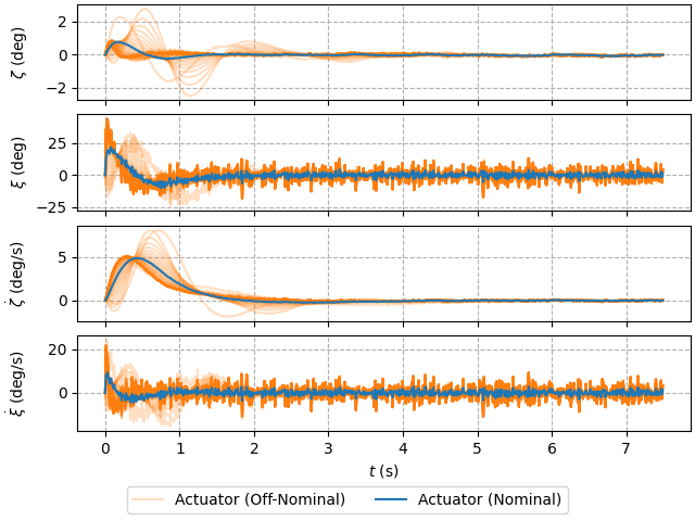
D-K iteration for non-square perturbation and simulation of perturbed systems
In this example, the perturbation Δ is non-square. In other words, the inputs and outputs of the perturbation are not identical. The orders are specified in a list. Once the robust controller is synthesized, it is tested on a set of perturbed systems by generating a set of perturbations Δ that have H-infinity norm less than or equal to 1.
In this example, a controller is designed for the linearized lateral dynamics of an aircraft from an example given in Section 14.1 of [M04].
"""D-K iteration with nonsquare perturbations

D-K iteration with a fixed number of iterations and fit order and closed-loop
simluation of perturbed models for the linearized lateral dynamics of an
aircraft.

The quantities of interest in the aircraft dynamics are shown below.

Airframe States
---------------
phi: Roll angle
beta: Sideslip angle
p: Roll rate
r: Yaw rate

Control Inputs
--------------
zeta: Rudder angle input
xi: Aileron angle input

Disturbances
------------
beta_w: Sideslip angle wind disturbance
p_w: Roll rate wind disturbance

Tracking Reference
------------------
phi_ref: Roll angle reference
"""

import numpy as np
import control
from matplotlib import pyplot as plt

import dkpy


def example_dk_iter_list_order_aircraft():
    # Example parameters
    eg = dkpy.utilities.example_mackenroth2004_p430()
    plant_gen = eg["P"]

    n_u = eg["n_u"]
    n_y = eg["n_y"]
    n_u_delta = eg["n_u_delta"]
    n_y_delta = eg["n_y_delta"]
    n_w = eg["n_w"]
    n_z = eg["n_z"]

    # Frequency
    freq_min = 0.01
    freq_max = 100
    num_freq = 100
    freq = np.logspace(np.log10(freq_min), np.log10(freq_max), num_freq)
    omega = 2 * np.pi * freq

    # DK-iteration controller synthesis
    dk_iter = dkpy.DkIterListOrder(
        controller_synthesis=dkpy.HinfSynLmi(
            lmi_strictness=5e-7,
            solver_params=dict(
                solver="MOSEK",
                eps=5e-8,
            ),
        ),
        structured_singular_value=dkpy.SsvLmiBisection(
            bisection_atol=1e-5,
            bisection_rtol=1e-5,
            max_iterations=1000,
            lmi_strictness=1e-7,
            solver_params=dict(
                solver="MOSEK",
                eps=1e-9,
            ),
        ),
        d_scale_fit=dkpy.DScaleFitSlicot(),
        fit_orders=[4, 4, 4],
    )
    # Alternative MATLAB block structure description
    # block_structure = np.array([[n_u_delta, n_y_delta], [n_w, n_z]])
    block_structure = [
        dkpy.ComplexFullBlock(n_y_delta, n_u_delta),
        dkpy.ComplexFullBlock(n_w, n_z),
    ]
    controller, N, mu, iter_results, info = dk_iter.synthesize(
        plant_gen,
        n_y,
        n_u,
        omega,
        block_structure,
    )
    controller.set_inputs(["phi_ref", "phi_meas", "beta_meas", "p_meas", "r_meas"])
    controller.set_outputs(["zeta_c", "xi_c"])
    print("mu:", mu)

    # Plot - DK-iteration results
    fig, ax = plt.subplots()
    for i, ds in enumerate(iter_results):
        dkpy.plot_mu(ds, ax=ax, plot_kw=dict(label=f"iter{i}"))

    # Generate off-nominal models with different perturbations
    delta_block_list = []
    # Nominal system uncertainty (no perturbation)
    delta_block = control.StateSpace([], [], [], [[0, 0], [0, 0]])
    delta_block.set_inputs(delta_block.ninputs, "y_del")
    delta_block.set_outputs(delta_block.noutputs, "u_del")
    delta_block_list.append(delta_block)
    # Constant gain perturbation
    num_offnom_gain = 20
    for gain_unc in np.linspace(-1, 1, num_offnom_gain):
        delta = control.StateSpace([], [], [], [gain_unc])
        delta_block = control.append(delta, delta)
        delta_block.set_inputs(delta_block.ninputs, "y_del")
        delta_block.set_outputs(delta_block.noutputs, "u_del")
        delta_block_list.append(delta_block)
    # Phase perturbation
    a_min = 0.01
    a_max = 10
    num_offnom_phase = 20
    for a in np.linspace(a_min, a_max, num_offnom_phase):
        delta_block = control.append(
            control.tf([1 / a, -1], [1 / a, 1]),
            control.tf([a, -1], [a, 1]),
            name="delta_block",
        )
        delta_block.set_inputs(delta_block.ninputs, "y_del")
        delta_block.set_outputs(delta_block.noutputs, "u_del")
        delta_block_list.append(delta_block)

    # Closed-loop simulation system
    input_id_sim_list = [
        "phi_ref",
        "beta_w",
        "p_w",
        "n[0]",
        "n[1]",
        "n[2]",
        "n[3]",
    ]
    output_id_sim_list = [
        "phi",
        "beta",
        "p",
        "r",
        "zeta_c",
        "xi_c",
        "zeta",
        "xi",
        "rate_xi",
        "rate_zeta",
    ]

    # Uncertain closed-loop system
    airframe = eg["airframe"]
    actuator = eg["actuator"]
    weight_unc = eg["weight_unc"]
    sum_noise = eg["sum_noise"]
    sum_uncertainty = eg["sum_uncertainty"]
    closed_loop_sim_list = []
    for delta_block in delta_block_list:
        closed_loop_sim = control.interconnect(
            syslist=[
                airframe,
                actuator,
                controller,
                weight_unc,
                delta_block,
                sum_noise,
                sum_uncertainty,
            ],
            inplist=input_id_sim_list,
            outlist=output_id_sim_list,
            name="closed_loop_sim",
        )
        closed_loop_sim.set_inputs(input_id_sim_list)
        closed_loop_sim.set_outputs(output_id_sim_list)
        closed_loop_sim_list.append(closed_loop_sim)

    # Time
    time_min = 0
    time_max = 7.5
    dt = 0.01
    num_time = round((time_max - time_min) / dt)
    time = np.arange(time_min, time_max, dt)
    # Reference signal
    phi_ref = 6 * np.ones_like(time)
    # Disturbance signals
    beta_w = np.zeros_like(time)
    p_w = np.zeros_like(time)
    # Sensor noise signals (assume sensors have identical noise characteristics)
    mean_noise = 0
    std_noise = 0.005
    noise_phi = np.random.normal(mean_noise, std_noise, num_time)
    noise_beta = np.random.normal(mean_noise, std_noise, num_time)
    noise_p = np.random.normal(mean_noise, std_noise, num_time)
    noise_r = np.random.normal(mean_noise, std_noise, num_time)
    # Exogenous input signal
    inputs_sim = np.array(
        [phi_ref, beta_w, p_w, noise_phi, noise_beta, noise_p, noise_r]
    )

    # Simulation response
    trd_sim_list = control.forced_response(
        sysdata=closed_loop_sim_list, T=time, U=inputs_sim
    )

    # Plot - Reference signal
    fig, ax = plt.subplots(layout="constrained")
    ax.plot(time, phi_ref)
    ax.set_ylabel("$\\phi_r$ (deg)")
    ax.set_xlabel("$t$ (s)")
    ax.grid(linestyle="--")

    # Plot - Disturbance signals
    fig, ax = plt.subplots(2, layout="constrained", sharex=True)
    ax[0].plot(time, beta_w)
    ax[1].plot(time, p_w)
    ax[0].set_ylabel("$\\beta_w$ (deg)")
    ax[0].grid(linestyle="--")
    ax[1].set_ylabel("$p_w$ (deg)")
    ax[1].grid(linestyle="--")
    ax[-1].set_xlabel("$t$ (s)")
    fig.align_ylabels()

    # Plot - Noise signals
    fig, ax = plt.subplots(4, layout="constrained", sharex=True)
    ax[0].plot(time, noise_phi)
    ax[1].plot(time, noise_beta)
    ax[2].plot(time, noise_p)
    ax[3].plot(time, noise_r)
    ax[0].set_ylabel("$n_{\\phi}$ (deg)")
    ax[1].set_ylabel("$n_{\\beta}$ (deg)")
    ax[2].set_ylabel("$n_{p}$ (deg/s)")
    ax[3].set_ylabel("$n_{r}$ (deg/s)")
    ax[-1].set_xlabel("$t$ (s)")
    for a in ax:
        a.grid(linestyle="--")
    fig.align_ylabels()

    # Plot - Output signals
    fig, ax = plt.subplots(4, layout="constrained", sharex=True)
    # Reference signal
    ax[0].plot(time, phi_ref, color="black", linestyle="--", label="Reference")
    for idx_sim, trd_sim in enumerate(reversed(trd_sim_list)):
        # Output signals
        phi = trd_sim.y[0, :]
        beta = trd_sim.y[1, :]
        p = trd_sim.y[2, :]
        r = trd_sim.y[3, :]
        # Plot signals (nominal)
        if idx_sim == len(trd_sim_list) - 1:
            ax[0].plot(time, phi, color="tab:blue", label="Nominal")
            ax[1].plot(time, beta, color="tab:blue", label="Nominal")
            ax[2].plot(time, p, color="tab:blue", label="Nominal")
            ax[3].plot(time, r, color="tab:blue", label="Nominal")
        # Plot signals (off-nominal)
        else:
            ax[0].plot(time, phi, color="tab:orange", alpha=0.25, label="Off-Nominal")
            ax[1].plot(time, beta, color="tab:orange", alpha=0.25, label="Off-Nominal")
            ax[2].plot(time, p, color="tab:orange", alpha=0.25, label="Off-Nominal")
            ax[3].plot(time, r, color="tab:orange", alpha=0.25, label="Off-Nominal")
    ax[0].set_ylabel("$\\phi$ (deg)")
    ax[1].set_ylabel("$\\beta$ (deg)")
    ax[2].set_ylabel("$p$ (deg/s)")
    ax[3].set_ylabel("$r$ (deg/s)")
    ax[-1].set_xlabel("$t$ (s)")
    for a in ax:
        a.grid(linestyle="--")
    handles, labels = ax[0].get_legend_handles_labels()
    legend_dict = dict(zip(labels, handles))
    fig.align_ylabels()
    fig.legend(
        handles=legend_dict.values(),
        labels=legend_dict.keys(),
        loc="outside lower center",
        ncol=3,
    )

    # Plot - Input signals
    fig, ax = plt.subplots(4, layout="constrained", sharex=True)
    for idx_sim, trd_sim in enumerate(reversed(trd_sim_list)):
        # Control signals
        zeta = trd_sim.y[6, :]
        xi = trd_sim.y[7, :]
        rate_zeta = trd_sim.y[8, :]
        rate_xi = trd_sim.y[9, :]
        if idx_sim == len(trd_sim_list) - 1:
            ax[0].plot(
                time, zeta, color="tab:blue", linestyle="-", label="Actuator (Nominal)"
            )
            ax[1].plot(
                time,
                rate_zeta,
                color="tab:blue",
                linestyle="-",
                label="Actuator (Nominal)",
            )
            ax[2].plot(
                time, xi, color="tab:blue", linestyle="-", label="Actuator (Nominal)"
            )
            ax[3].plot(
                time,
                rate_xi,
                color="tab:blue",
                linestyle="-",
                label="Actuator (Nominal)",
            )
        else:
            ax[0].plot(
                time,
                zeta,
                color="tab:orange",
                alpha=0.25,
                linestyle="-",
                label="Actuator (Off-Nominal)",
            )
            ax[1].plot(
                time,
                rate_zeta,
                color="tab:orange",
                alpha=0.25,
                linestyle="-",
                label="Actuator (Off-Nominal)",
            )
            ax[2].plot(
                time,
                xi,
                color="tab:orange",
                alpha=0.25,
                linestyle="-",
                label="Actuator (Off-Nominal)",
            )
            ax[3].plot(
                time,
                rate_xi,
                color="tab:orange",
                alpha=0.25,
                linestyle="-",
                label="Actuator (Off-Nominal)",
            )
    ax[0].set_ylabel("$\\zeta$ (deg)")
    ax[1].set_ylabel("$\\xi$ (deg)")
    ax[2].set_ylabel("$\\dot{\\zeta}$ (deg/s)")
    ax[3].set_ylabel("$\\dot{\\xi}$ (deg/s)")
    ax[-1].set_xlabel("$t$ (s)")
    for a in ax:
        a.grid(linestyle="--")
    handles, labels = ax[0].get_legend_handles_labels()
    legend_dict = dict(zip(labels, handles))
    fig.align_ylabels()
    fig.legend(
        handles=legend_dict.values(),
        labels=legend_dict.keys(),
        loc="outside lower center",
        ncol=2,
    )
    plt.show()


if __name__ == "__main__":
    example_dk_iter_list_order_aircraft()
Output:
mu: 0.9824275970458984
After the controller is synthesized, a set of off-nominal models are generated by interconnecting various admissible perturbations Δ with the nominal model. Then, the closed-loop systems are formed for each perturbed system. The time domain response of the systems can be obtained for a step response in the roll angle reference signal, no external disturbances, and moderate sensor noise. In particular, the response of the system states and actuator inputs are shown.
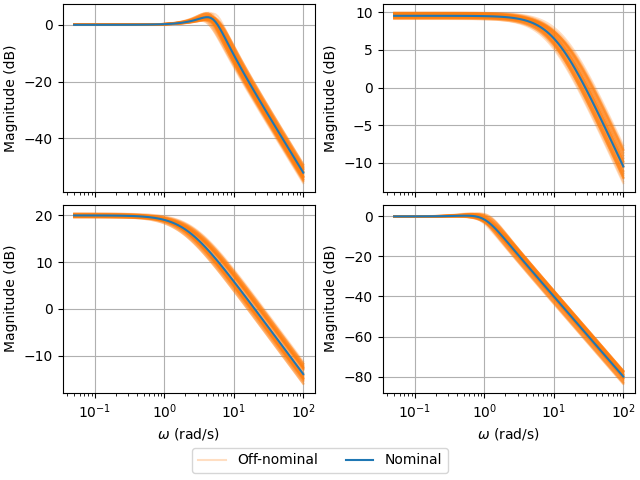
Multi-Model Uncertainty Characterization: Academic Model
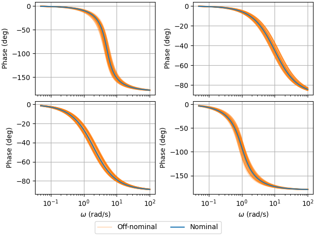
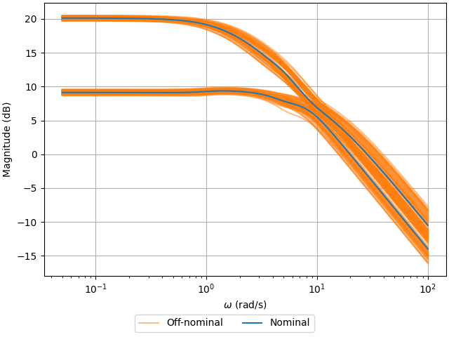
In this example, an unstructured uncertainty set is characterized from a set of nominal and off-nominal frequency responses. This is an academic example as the uncertain model in this problem is arbitrarily selected for the purpose of demonstration. The off-nominal models are generated from a nominal model by randomly perturbing the parameters within a known bound.
"""Multi-model uncertainty characterization from frequency response data."""

from matplotlib import pyplot as plt

import dkpy


def example_uncertainty_characterization():
    """Multi-model uncertainty characterization from frequency response data."""

    # Load example data
    eg = dkpy.example_multimodel_uncertainty()
    response_nom = eg["complex_response_nominal"]
    response_offnom_list = eg["complex_response_offnominal_list"]
    omega = eg["omega"]

    # Uncertainty models
    uncertainty_models = {
        "additive",
        "multiplicative_input",
        "multiplicative_output",
        "inverse_additive",
        "inverse_multiplicative_input",
        "inverse_multiplicative_output",
    }

    # Compute uncertainty residual frequency response
    response_residuals_dict = dkpy.compute_uncertainty_residual_response(
        response_nom,
        response_offnom_list,
        uncertainty_models,
    )

    # Compute uncertainty weight frequency response
    response_weight_left, response_weight_right = (
        dkpy.compute_uncertainty_weight_response(
            response_residuals_dict["inverse_additive"], "diagonal", "diagonal"
        )
    )

    # Fit overbounding stable and minimum-phase uncertainty weight system
    weight_left = dkpy.fit_uncertainty_weight(response_weight_left, omega, [4, 5])
    weight_right = dkpy.fit_uncertainty_weight(response_weight_right, omega, [3, 5])

    # Plot: Magnitude response of nominal and off-nominal systems
    dkpy.plot_magnitude_response_uncertain_model_set(
        response_nom,
        response_offnom_list,
        omega,
    )

    # Plot: Phase response of nominal and off-nominal systems
    dkpy.plot_phase_response_uncertain_model_set(
        response_nom,
        response_offnom_list,
        omega,
    )

    # Plot: Singular value response of nominal and off-nominal systems
    dkpy.plot_singular_value_response_uncertain_model_set(
        response_nom,
        response_offnom_list,
        omega,
    )

    # Plot: Singular value response of uncerainty residuals
    dkpy.plot_singular_value_response_residual(response_residuals_dict, omega)

    # Plot: Comparison of singular value response of uncerainty residuals for each
    # uncertainty model
    dkpy.plot_singular_value_response_residual_comparison(
        response_residuals_dict, omega
    )

    # Plot: Magnitude response of uncertainty weight frequency response and overbounding
    # fit
    dkpy.plot_magnitude_response_uncertainty_weight(
        response_weight_left,
        response_weight_right,
        omega,
        weight_left,
        weight_right,
    )
    plt.show()


if __name__ == "__main__":
    example_uncertainty_characterization()
dkpy provides plotting functionality for the nominal and off-nominal systems. The frequency response of the magnitude, phase, and singular values are as follows. These plots show the variation in the frequency response caused by the variation in parameters.
Next, the uncertainty residual can be computed for each off-nominal system and uncertainty model. dkpy implements six unstructured uncertainty models:
- Additive uncertainty (“A”);
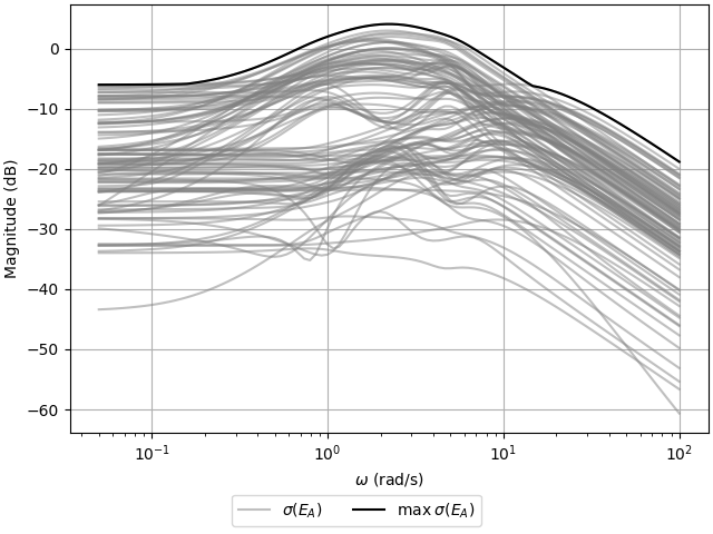
- Multiplicative input uncertainty (“I”);
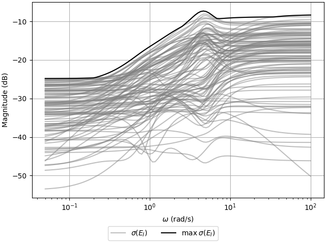
- Multiplicative output uncertainty (“O”);
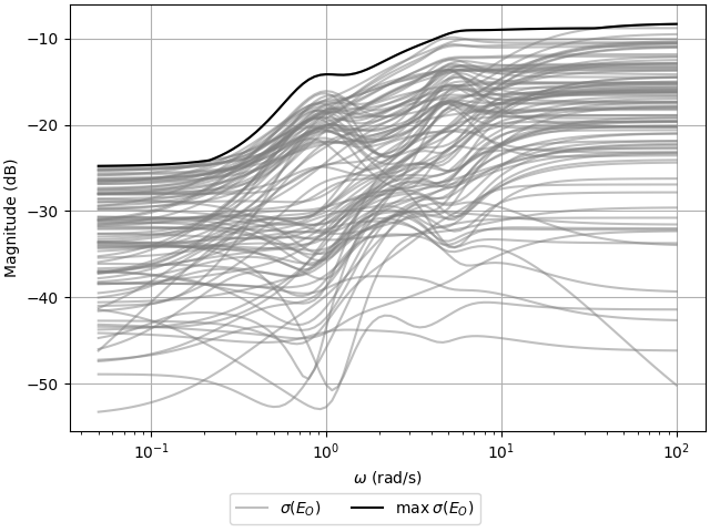
- Inverse additive uncertainty (“iA”);
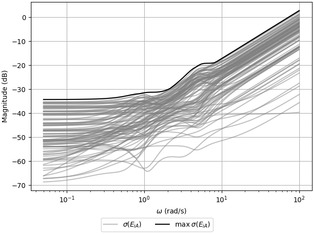
- Inverse multiplicative input uncertainty (“iI”);
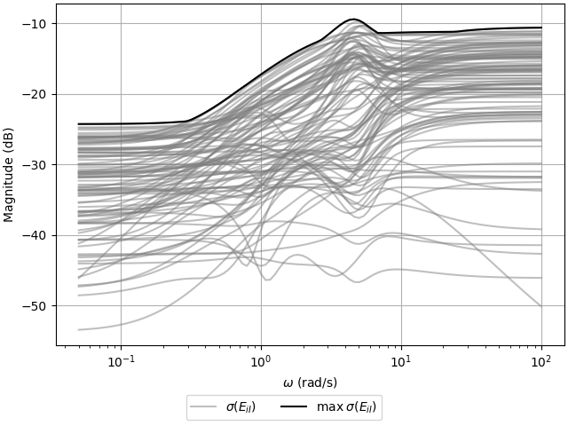
- Inverse multiplicative output uncertainty (“iO”).
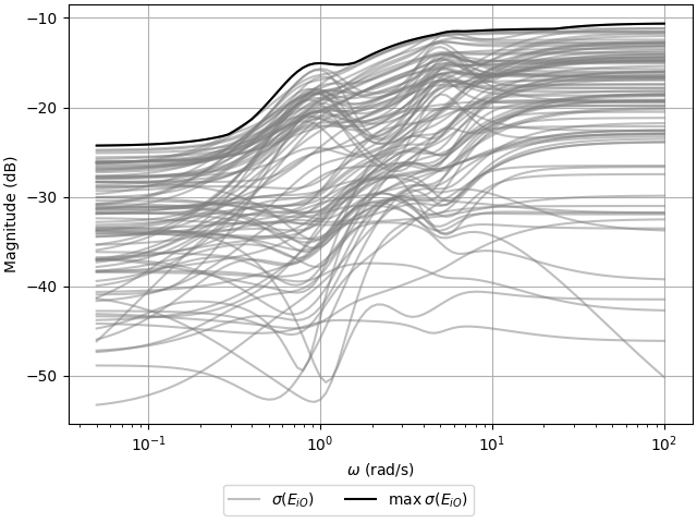
See Chapter 8.2.3 of [SP06] for more information on these unstructured uncertainty models. The maximum singular value responses of all uncertainty models are shown here.
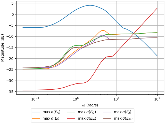
As a rule of thumb, the uncertainty model that is selected should have the smallest maximum singular value over the control bandwidth and high uncertainty at large frequencies to account for unmodeled dynamics. In this case, the inverse additive uncertainty (“iA”) model seems to be the best option, which will be used moving forward.
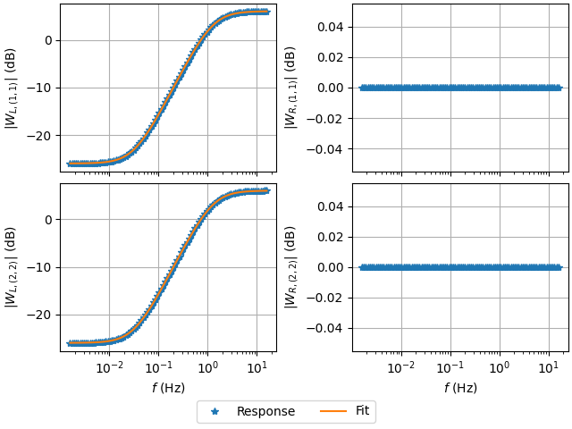
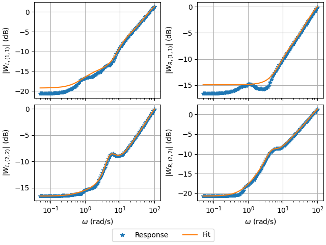
The uncertainty set is parametrized as E = WL Δ WR. E is the uncertainty residual, Δ is the normalized perturbation, and WL, WR are the dynamic weights used to parametrize the uncertainty set. The frequency response of the optimal weights with minimal magnitude at each frequency can be solved for from the uncertainty residuals for different assumptions on their structure. It is assumed that both weights are diagonal moving forward. Then, an overbounding stable and minimum phase linear time-invariant (LTI) system can be fit to the frequency response of the weights to obtain a LTI description of the uncertainty set. The optimal weight frequency responses and fitted weights are shown below.
Multi-Model Uncertainty Characterization: Aircraft Actuator Model
In this example, an unstructured uncertainty set is characterized from a set of nominal and off-nominal frequency responses. In this example, the uncertainty of an aircraft actuator model is characterized using an actuator model from an example given in Section 14.1 of [M04].
"""Multi-model aircraft actuator uncertainty characterization from frequency response
data.

"""

from matplotlib import pyplot as plt

import dkpy


def example_aircraft_uncertainty_characterization():
    """Multi-model aircraft actuator uncertainty characterization from frequency
    response data.
    """
    # Load example data
    eg = dkpy.example_aircraft_actuator_uncertainty()
    response_actuator = eg["response_actuator_nominal"]
    response_actuator_offnom_list = eg["response_actuator_offnominal"]
    omega = eg["omega"]

    # Compute the residual response for different uncertainty models
    response_residual = dkpy.compute_uncertainty_residual_response(
        response_actuator,
        response_actuator_offnom_list,
        {"additive", "multiplicative_input", "inverse_multiplicative_input"},
    )

    # Compute the optimal uncertainty weights with a given structure
    response_weight_left, response_weight_right = (
        dkpy.compute_uncertainty_weight_response(
            response_residual["multiplicative_input"],
            "scalar",
            "identity",
        )
    )

    # Fit an overbounding LTI system to the optimal uncertainty weight response
    weight_left = dkpy.fit_uncertainty_weight(response_weight_left, omega, 1)

    # Plot: Singular value response of nominal and off-nominal systems
    dkpy.plot_singular_value_response_uncertain_model_set(
        response_actuator, response_actuator_offnom_list, omega, hz=True
    )

    # Plot: Comparison of singular value response of uncerainty residuals for each
    # uncertainty model
    dkpy.plot_singular_value_response_residual_comparison(
        response_residual, omega, hz=True
    )

    # Plot: Magnitude response of uncertainty weight frequency response and overbounding
    # fit
    dkpy.plot_magnitude_response_uncertainty_weight(
        response_weight_left,
        response_weight_right,
        omega,
        weight_left=weight_left,
        hz=True,
    )
    plt.show()


if __name__ == "__main__":
    example_aircraft_uncertainty_characterization()
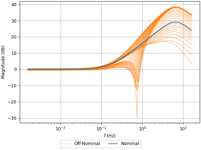
The off-nominal frequency response data is generated by sampling valid perturbations from the uncertainty model provided in the problem statement.
Three different candidate uncertainty models are evaluated: additive uncertainty, multiplicative input uncertainty, and inverse multiplicative input uncertainty. The multiplicative input uncertainty is selected as it yields the smallest residual singular values.
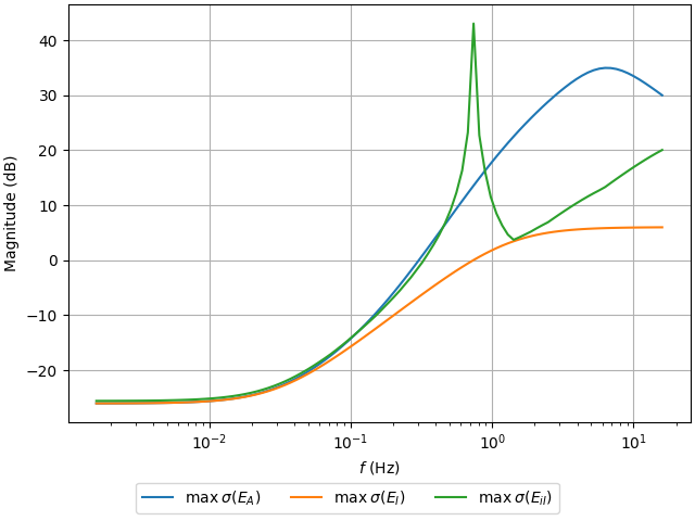
The left uncertainty weight is constrained to be scalar whereas the right uncertainty weight is constrained to the identity matrix. Given that the right uncertainty weight is the identity matrix, a fit does not need to be performed for this weight as it will be neglected in the generalized plant.